K-Pop Daisuki - Statistics and Probability applied to Kpop Videos

First things off.

Statistics and Probability do not give certainty, and they can be off, sometimes by a lot. For that reason, all numbers are estimates, and the best a model can do is calculate how precise and accurate it is. Past about 95% it gets exponentially harder to improve the model, and even a full-population model (one that uses 100% of the possible available data) cannot be 100% correct to predict future events.

What are Non-organic views?

Most Youtube views are viewed by people - that is a given. However, as the internet is made by exposition and unfortunately wrong impressions, people find ways to change the number of views to prove something, as if having more views somewhat proves a music is better or more popular. While this is harmless, it created a business (outside Youtube) of purchasing views. In the early 2010’s, that meant farms of computers or usually mobile phones repeating the video over and over, to boost the numbers. Youtube tries hard to ban these farms and any bots (we often get negative daily views when there is a big bot farm detected), but it is always an uphill battle, so Youtube did what can be considered both clever, and a little low: it created its own “legal” and cheap way to boost views - indirectly of course: With Youtube True-view. When you set a video as an advertisement, it will display on other people’s videos as such, and work as an ad - the thing is, those views count. So not only you advertise the video, you also gain views. "Worst" thing is, its not even that expensive, not for a company or a lot of engaged fans. 

We call non-organic views all those views that are somewhat not really from a person interested in the video, but from bots, view purchases or simply advertisements.

How can we know a video has Non-organic views?

The word Organic is self explanatory. It means it follows a very organic behavior. Videos have always behaved the same expected way: they get released, a lot of people watch the new content, and as time goes by the number of people watching (and views) falls. Not surprisingly, this fall is logarithmic, and while it might not be the same for every type of video, it is the same when we are talking about the exact same concept: Music Videos (or even more specific, Korean Music Videos). There are a few variations, but they are organic too: there are no sudden peaks or falls, but rather flow with how people watch. If you see a video having daily videos not following a logarithmic line, with sudden changes, something is up. Some times it might be that some really nice link made by someone famous went viral, but that is actually very rare. Almost always, it means non-organic views are at work: Bots started streaming, or more likely someone purchased ads for that video (anyone, not only the owner, can invest in advertisements on valid videos), or even external view harvesters were hired. It is easy to dismiss the idea that viewership is not as predictable as this, specially if you have never followed multiple (let alone thousands) of videos before, but they are. As seen in the graphics below (1a), even the Min-Max of hundreds of videos is not farther than 3σ (90.8% of total).

How do you detect normal logarithmic views? Is it real? Can we trust it?

Detection is easy: you merge all videos, calculate the means, work out standard deviations from the set, plot an histogram (how many times videos behave higher or lower the mean) and check if they are, indeed, following the same trend (quick answer: they are) to validate the model, then use simulation to improve the model by tweaking truncation and deviation values, rinse and repeat until the selected sample and accuracy aim stabilizes. You apply the basic tenets of Statistics and Probability and get a “standard model” (also called null hypothesis) that portrays the majority of videos; and then from the same mathematics involved, you have how accurate (how far off the mean it is) and precise (how far off the mean is from reality) this is. Using computer models (which is also part of Stat&Prob), you improve the approximation by removing known noise (videos that are clearly not behaving properly) and outliers (videos that are exceptions, either too high or too low) and apply other rules based on your findings (for instance, a daily view graphic results in a truncated normal curve, because you have no limit to how high views can go, but you have an absolute minimal value (zero)). If you want to go the extra mile for accuracy, you create a variable model that accounts for these exceptions (Videos with lower views, and videos with higher views).

How to build that model

For this, we will use data for September 14th, 2021 on kpop.daisuki.com.br (you can see TODAY’s analysis - automaticaly - on this page). The data we have are as follow:

• Total available videos to analyse (past year): 1859;
• Total eligible videos: 480

The reason we do not use all videos is because 1379 videos did not pass our quality check. The top 4 computed reasons were:

• Missing first day of daily views: 588
• Too little total views (less than 50.000): 365
• One or more Daily View per Like were absurd (above max deviation 3σ): 136
• One or more Daily Views were absurd (above max deviation 3σ): 107

While we end up with only 26% sample size, it is ok. According to Stat&Prob, a sample should be at least 10~30 per variable. We have 2 variables (views and likes), which brings to 20~60. Different methods will accept different intervals. For safety, we will use the higher standard and double it: 120. Therefore, we are 4 times above the minimum safe sample size. The reason sample sizes can be so small is because the whole mathematics behind Sampling Statistics is optimized for having small samples otherwise it would be really hard to get anything done other than using a full population, and besides, even with a full population you cannot reach 100% future prediction. Also, if the histogram proves our data falls in a Stat&Prob model (it does, it fits a truncated gaussian distribution), it is accounted for. Mathematically, a sample model only changes in how the mean and therefore precision is calculated.

With this, we can build the first average distribution of views and likes per day as follows (note, the images are from an earlier version, check this link for today’s live distribution)

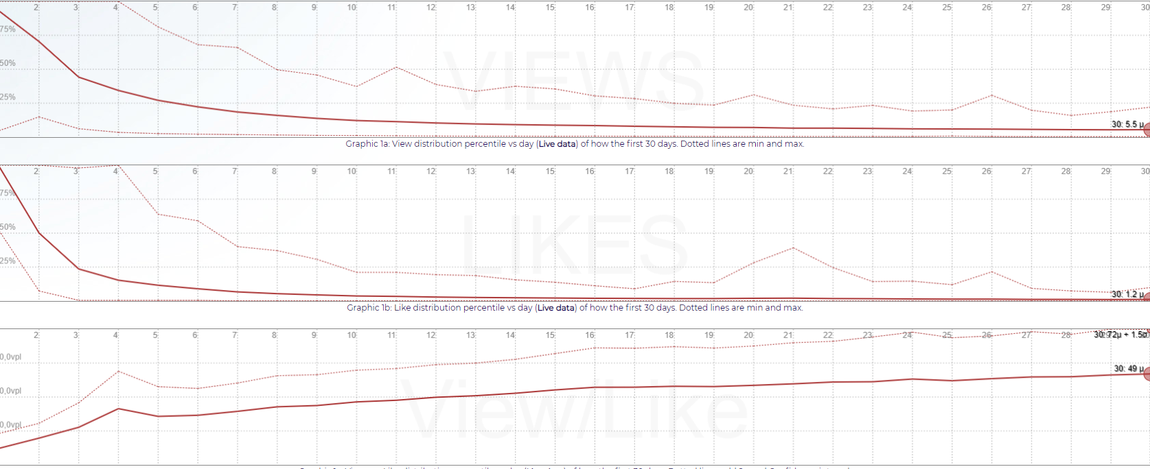
Graphic 1 - Views, Likes, and View per Like, per day from release

The graphic shows our three main interest points: Views, Likes and Views per Like. The dotted line in Views and Likes represent the min and maximum values, while the dotted line in View per Like adds 2σ and confidence interval (that means all values below it represent 97.7% of the cases, since there is no under-prediction)

But how sure are we that all videos are represented? It turns out very. If we build an histogram of every day for every data, we get a very tight match with a normal curve. The following show days 2, 6 and 12 histograms (image is of an older version, check this link for today’s live distribution)

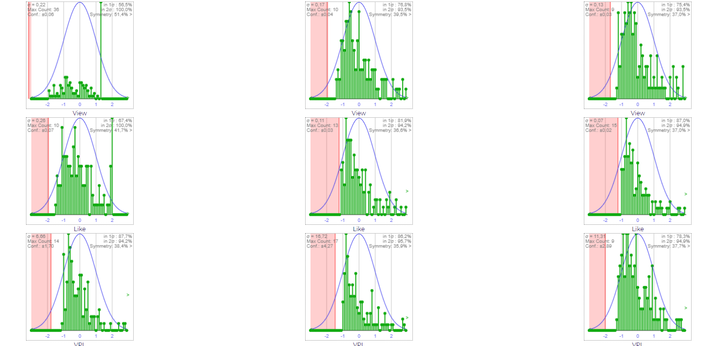
Graphic 2 - Histograms

The red area represents zero views, likes or view per like, which cannot happen, which explains why we are using a truncated gaussian approach. In order to understand what a gauss/normal (or Bell Curve) graph means, check the following image. The standard deviation (σ) is how far a value is off the mean (μ). In a gaussian curve, the percentage of times values will fall under each Z-score (standard deviation) is give below. Since this is a truncated gaussian were every value below is included, we use the Cumulative percent, this, 97.7% of all values (in our case, videos) will be under 2σ. From the graphic above, you will notice that is indeed the case (note the second information on the right side of each graphic, which is how many videos are under 2σ).

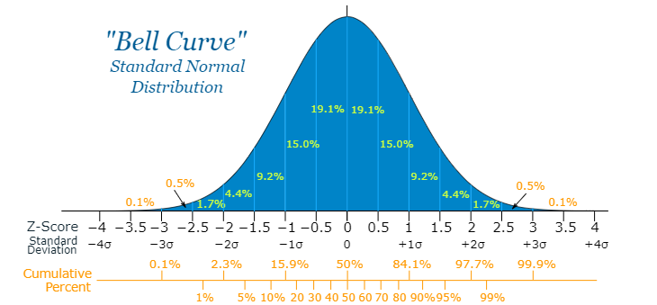
Graphic 3 - Distribution and probabilities in a Gauss Curve

In order to work with the truncated curve, we basically “truncate” the sample by removing the same amount of outliers from each side. A common approach is the Interquartile Range, which cuts 25% of each side (so you end up with 50% of the original values), but we don’t need that much to keep our symmetry (number of entries on each side), so we are using as time of writing 5%. This means that from the 480 initial videos, we cut 24 from each side, ending up with 432 videos (23% of the available and still 3.6 times higher than minimum safe sample). Truncated ranges are useful even on symmetric distributions because it removes the noise of outliers, and because it actually increases the precision of the model, its use is very common in any statistical model.

So how do you use and reach conclusions?

Since our goal is to take into consideration videos with low and high views, we build 3 models: one for low views (~500.000- total), one for average views (500.000~1.300.000 total) and one for high views (1.300.000+~) views. The method to extract the power law regression formula is using regressed formulas either manually or from an application such as Excel or Mathlab. A power law looks like “a * xb”. Using the regressed formula from our plots (as of September 14th 2021), we have the following View per Like formulas:

Vpl = 23 * day 0.34 For low view videos
Vpl = 13 * day 0.44 For medium view videos
Vpl = 25 * day 0.37 For high view videos

The following graphic shows the videos broken in 4 sizes (old image, check this link for today’s live data)

Graphic 4 - Views, Likes and View per Like broken up in 4 groups

We use a quadratic formula to approach the formulas in the intervals as needed. For the expected daily view distribution, for use in the view behavior method, we have the following single formula:

Views = 1.03 * day -0.92

These formulas are just the mathematical forms of the graphics shown earlier.

All of the above formulas already include 1.5 standard deviation and confidence intervals, bringing their accuracy to 95% and precision to 95%

Expected variations

There are a few things we know from the behavior of videos that are lost on the flattening of averages, one of it can be seen in the graphics above and is highlighted below:

Graphic 5 - 4th day Anomaly

This strange bump in views (and likes) happens so often on the 4th day that even with a big sample, it is still there. Evaluating the reason, we come to a simple conclusion: the 4th day is, on average, the first Sunday after release. We can therefore improve our model to expect that, by allowing more Views per Like, and Views, on the first Sunday (the graphic shows it as the 4th day, but since we figured its caused by the first Sunday, we can actually calculate it on the proper day on a video-per-video basis). It affects both View per Like and Views methods. Notice that adding allowances into the model, we are making it more prone to false negatives (not detect non-organic views), but that is just a caution approach since we want to avoid false positives (point to non-organic views that are actually organic).

Another expected anomaly is that some videos can have extremely high views on the first and even second days way above the average (we already saw that on the View formula, which instead of starting with a 100% daily view on the first day, resulted on a mathematical impossibility of 103%. To fix it, we account for possible extra views on the first day, and some on the second day.

Other anomalies

We also analyzed videos to check for other possible variations, and while there are small changes, they are not statistically significant. For instance, Female and Male videos:

Graphic 6 - Views per Like for Female and Males (Green is low like videos, Red is high likes. Dotted is maximums)

There were also not much change in Group and Solo videos.

The final math to calculate Non-organic views

• The known non-organic views are based on Youtube charts, which use a Friday-to-thursday week. This means we also have to use those 7 day blocks;
• Because we cannot crosscheck all non-organic views if a video does not chart, it is expected that in several videos the crosschecked non-organic views will always be smaller than actually they are;
• We should take into consideration our findings about the 4th (or rather, first sunday) day;
• Our model incorporates as an average the fact that some videos have the highest views in the second day, but does not quantify it. For that reason, we take the data that only 90% of videos have the highest views in the first day into consideration by “forgiving” a small part of views in the first day (~10%);
• Once we confirmed why the 4th day have a different VpL, we can use the Precision predictor to improve our estimates: instead of using just the average (95% accuracy but 0% precision), we will use average + 1.5σ (95% accuracy and 95% precision);

By applying both methods (View per Like or View behavior), we come to similar results, where some outlier videos can show variations. View per Likes have a better day-per-day precision and can be calculated starting on the first day since it does not require us to find the normal curve to apply, while the View behaviour method has the benefit of allowing us to detect non-organic views on videos without likes.

Because the View method does not include the 1.5σ standard deviation accuracy boost, it will usually calculate a small extra number of Non-organic views. That is on purpose to compensate for the lost Non-organic views from the VpL method because it is truncated.

It is not magic, its science.